Long SQL statements have a way of growing unreadable. Subqueries nest three deep, the same aggregate gets computed in four places, and six months later nobody remembers what the query does. Two features fix most of this: Common Table Expressions and window functions. They cut repetition, make intent obvious, and in many cases replace slow self-joins with a single pass over the data. This post walks through both in PostgreSQL, with runnable examples on a small orders table.
Start with the schema and some rows:
CREATE TABLE orders (region VARCHAR(100), amount INT, product VARCHAR(100));

INSERT INTO orders (region, amount, product)
VALUES ('EU', 10, 'Product1'),
       ('EU', 20, 'Product2'),
       ('US', 1,  'XYZ'),
       ('JP', 10, 'ABC');
Common Table Expressions
A Common Table Expression (CTE), written with the WITH keyword, defines a named temporary result set that exists for the duration of a single query. Think of it as a scratch table you reference by name. A CTE can wrap SELECT, INSERT, UPDATE, or DELETE, though SELECT is the common case.
Say you want products from regions that account for at least 10% of total sales. Written as nested subqueries, that becomes hard to follow:
SELECT region, product,
       (SELECT SUM(amount) FROM orders AS o2 WHERE o2.region = o.region) AS total_sales
FROM orders AS o
WHERE region IN (
    SELECT region
    FROM orders
    GROUP BY region
    HAVING SUM(amount) > (SELECT SUM(amount) FROM orders) / 10
);
The same logic recomputes sums, mixes filtering with calculation, and hides the threshold deep inside a HAVING. The CTE version reads top to bottom, one step per block:
WITH total AS (
    SELECT SUM(amount) / 10 AS threshold
    FROM orders
),
sales_by_region AS (
    SELECT region, SUM(amount) AS total_sales
    FROM orders
    GROUP BY region
),
top_regions AS (
    SELECT region
    FROM sales_by_region
    WHERE total_sales > (SELECT threshold FROM total)
)
SELECT o.region, o.product, s.total_sales
FROM orders AS o
JOIN sales_by_region AS s ON s.region = o.region
WHERE o.region IN (SELECT region FROM top_regions);
Each name describes what it holds. The flow is linear instead of nested, and you can read it without unwinding three levels of parentheses.
CTEs also do something plain subqueries cannot: they can reference themselves. A recursive CTE has an anchor term, a UNION ALL, and a recursive term that reads the CTE's own output. This generates the numbers 1 through 100:
WITH RECURSIVE numbers(n) AS (
    VALUES (1)
    UNION ALL
    SELECT n + 1 FROM numbers WHERE n < 100
)
SELECT n FROM numbers;
The same pattern walks hierarchies - an employees table with a manager_id, a category tree, a graph of dependencies.
One performance note that trips people up. Before PostgreSQL 12, a CTE was always an optimization fence: it was materialized in full, and the planner could not push outer filters down into it. Since version 12, a non-recursive, side-effect-free CTE referenced exactly once is inlined into the parent query by default, so it plans like an ordinary subquery. You can force the old behavior with WITH name AS MATERIALIZED (...) when you actually want to compute a result once and reuse it, or push the other way with NOT MATERIALIZED. Recursive CTEs and CTEs referenced multiple times are still materialized.
Window Functions
A window function computes a value across a set of rows related to the current row, without collapsing them. That is the difference from a GROUP BY aggregate: the rows stay separate, but each one can carry a value derived from its group.
Total sales per region, attached to every row:
SELECT region, product,
       SUM(amount) OVER (PARTITION BY region) AS total_sales
FROM orders;
PARTITION BY region splits the rows into groups; SUM(amount) runs over each group. Every EU row shows 30, every US row shows 1. Add ORDER BY inside the OVER clause to rank within a partition:
SELECT region, product,
       SUM(amount) OVER (PARTITION BY region) AS total_sales,
       RANK() OVER (PARTITION BY region ORDER BY amount DESC) AS sales_rank
FROM orders;
RANK() numbers rows by descending amount within each region. Its cousins matter when there are ties: ROW_NUMBER() always gives distinct numbers, RANK() leaves gaps after a tie (1, 1, 3), and DENSE_RANK() does not (1, 1, 2). Other useful ones are LAG and LEAD for the previous and next row, and FIRST_VALUE, LAST_VALUE, and NTH_VALUE for positional lookups. Plain aggregates - SUM, MIN, MAX, AVG - all work as window functions too.
The frame clause controls which rows the function sees. When you add ORDER BY without a frame, the default is RANGE BETWEEN UNBOUNDED PRECEDING AND CURRENT ROW, meaning the frame runs from the partition start to the current row and its peers. That default is why LAST_VALUE so often surprises people: it returns the current row rather than the partition's last row, because the frame ends at the current row. To look at the whole partition, set the frame explicitly with ROWS BETWEEN UNBOUNDED PRECEDING AND UNBOUNDED FOLLOWING. ROWS counts physical rows; RANGE groups rows with equal ORDER BY values together as peers.
Practical Examples
Top-N per group. Rank within each region, then filter. A CTE keeps it readable because you cannot reference a window function's result in a WHERE clause directly:
WITH ranked_orders AS (
    SELECT region, product, amount,
           ROW_NUMBER() OVER (PARTITION BY region ORDER BY amount DESC) AS rn
    FROM orders
)
SELECT region, product, amount
FROM ranked_orders
WHERE rn <= 3;
Use ROW_NUMBER() for a hard cap of N rows, RANK() or DENSE_RANK() when ties should all qualify.
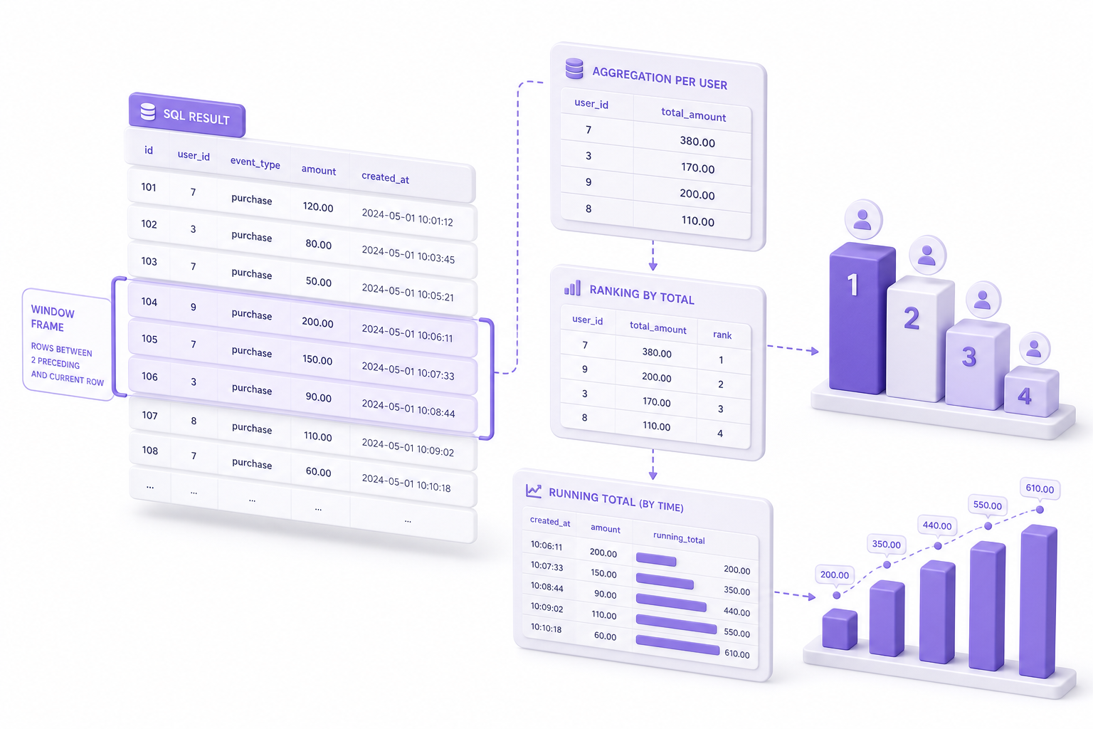
Running totals. Add ORDER BY inside OVER and the default frame turns the aggregate into a cumulative one:
SELECT region, product, amount,
       SUM(amount) OVER (PARTITION BY region ORDER BY amount) AS running_total
FROM orders;
Each row sums itself and everything before it in the ordered partition.
Difference between adjacent rows. LAG reaches back one row, so subtracting gives the delta from the previous product:
SELECT region, product, amount,
       amount - LAG(amount, 1) OVER (PARTITION BY region ORDER BY amount) AS diff_from_prev
FROM orders;
The first row in each partition has no predecessor, so LAG returns NULL; pass a third argument, LAG(amount, 1, 0), for a default. LEAD does the same looking forward.
A Note on Performance
The big win is that window functions replace correlated subqueries and self-joins. The classic "total per region on every row" written with a self-join scans the table once per group; the OVER (PARTITION BY region) version sorts once and streams through. On a table of millions of rows that difference is large.
CTEs are not free, though. A materialized CTE - recursive, referenced more than once, or marked MATERIALIZED - is computed and stored before the outer query runs, and the planner cannot push filters into it. If a CTE produces a wide intermediate result that the outer query barely touches, that materialization can cost more than the repetition it was meant to avoid. The fix is usually to let PostgreSQL inline it (the default for single-reference CTEs in 12 and later) or to restructure so the expensive work happens after filtering. Window functions carry a sort cost as well: each distinct PARTITION BY/ORDER BY combination can require its own sort, and on large partitions that shows up in the plan.
Check EXPLAIN (ANALYZE, BUFFERS) before assuming a rewrite is faster. The query that reads best is not always the one that runs best, and a window function over a poorly indexed sort key can spill to disk. This is also where these patterns quietly degrade in production: a CTE that inlined fine on test data starts materializing a huge intermediate as tables grow, or a window sort that fit in work_mem begins spilling. Pulse watches query plans and execution stats over time, so when a once-cheap window query turns into your slowest endpoint, you see the regression and its root cause instead of guessing.
CTEs and window functions are mostly a readability and correctness tool, with performance gains as a frequent bonus. Reach for a CTE when nesting hurts comprehension, a recursive CTE when you need to walk a hierarchy, and a window function whenever you find yourself joining a table to itself just to attach a group-level number. Confirm the result with EXPLAIN and you get queries that are easier to maintain and, more often than not, faster.